4. More taylor series

4.1. Exponentials

4.1.1. The number \(e\): base for natural exponentials and logarithms

In earlier lessons we discussed the exponential function at length. Here we discuss some of the reasons for which we consider Euler’s number \(e\) to be the “natural” base for exponentials and logarithms, analogously to how radians are the natural unit of measure for circles.

Part of this is a visual exploration of \(e^x\) and an graphical look at its slope, to then conclude that:

\[\frac{d e^x}{dx} = e^x\]

which is not true for other bases, like \(2^x\) and \(10^x\)

We can also mention that:

\[e = \lim_{n \rightarrow \infty} \left(1 + \frac{1}{n}\right)^n\]

and calculate it for values of n like 1, 10, 100, 1000, 10000, … We can also calculate \(e\) with:

\[e = \frac{1}{0!} + \frac{1}{1!} + \frac{1}{2!} + \frac{1}{3!} + \frac{1}{4!} + \frac{1}{5!} + \dots = \sum_{k=0}^{\infty} \frac{1}{k!} \approx 2.71828182846\]

but the justification for that will only come when we show how to calculate the Taylor series for \(e^x\).

Caution

It is also worth mentioning that difference communities in math, science, and engineering use \(\log(x)\) to mean the natural logarithm (base \(e\)). Other communities will use \(\log(x)\) to mean the base 10 logarithm, and they say \(\ln(x)\) for the natural logarithm. I use the former approach, and the various programming language libraries (C, Python, …) do the same.

But we take a break from these notes as we get to use a proper text book to explore exponentials and logarithms in more detail.

4.1.2. The Taylor series for \(e^x\) – visually

First we look at it visually. We will want to plot terms in the following way in gnuplot and geogebra and desmos:

$ gnuplot
## then the following lines have the prompt gnuplot> and we type:
reset
set grid
set xrange [-1:3]
set terminal qt linewidth 3
plot exp(x) lw 2
replot 1
replot 1 + x
replot 1 + x + x**2 / 2!
replot 1 + x + x**2 / 2! + x**3 / 3!
replot 1 + x + x**2 / 2! + x**3 / 3! + x**4 / 4!
replot 1 + x + x**2 / 2! + x**3 / 3! + x**4 / 4! + x**5 / 5!
replot 1 + x + x**2 / 2! + x**3 / 3! + x**4 / 4! + x**5 / 5! + x**6 / 6!

In geogebra or desmos:

e^x
1
1 + x
1 + x + x**2 / 2!
1 + x + x**2 / 2! + x**3 / 3!
1 + x + x**2 / 2! + x**3 / 3! + x**4 / 4!
1 + x + x**2 / 2! + x**3 / 3! + x**4 / 4! + x**5 / 5!
1 + x + x**2 / 2! + x**3 / 3! + x**4 / 4! + x**5 / 5! + x**6 / 6!

While looking at the visual output I discuss with the students how the polynomial approximations look different to the left and to the right of the origin: to the right the polynomials all approximate from below, while to the left the even/odd alternating polynomials approximate from above/below respectively.

4.1.3. The Taylor series for \(e^x\) – calculating the coefficients

Remembering that \(\frac{de^x}{dx} = e^x\) we can calculate:

\[\frac{d^k e^x}{dx^k} \bigg \rvert_{x = 0} = e^0 = 1\]

which gives us Taylor coefficients \(a_k = \frac{1}{k!}\) and the series looks like:

\[e^x = \sum_{k=0}^{\infty} \frac{x^k}{k!} = 1 + x + \frac{x^2}{2!} + \frac{x^3}{3!} + \frac{x^4}{4!} + \dots\]

Here I usually spend some time discussing how the \(k!\) on the denominator makes this series converge, even when \(x^k\) can get really big. Later I will contrast that with other denominators and we should make sure we are always that the series will converge.

I also often take off on another tangent here: I write out the series for \(e^x\) and underneath it I write the series for \(\cos(x)\) and \(\sin(x)\). In doing this I align all the terms so it looks like this:

\begin{align*} e^x =& \; 1 & + x & + \frac{x^2}{2!} & + \frac{x^3}{3!} & + \frac{x^4}{4!} & + \frac{x^5}{5!} & + \dots \\ \cos(x) =& \; 1 & {} & - \frac{x^2}{2!} & {} & + \frac{x^4}{4!} &{} & + \dots \\ \sin(x) =& \; {} & x & {} & - \frac{x^3}{3!} & {} & + \frac{x^5}{5!} & + \dots \end{align*}

I then have them speculate on whether it looks like the exponential series might contain the \(sin()\) and \(cos()\) series, but with funny alternations of + and - signs.

It’s hard to get that alternation, but I show that if you take the series for \(e^{ix}\) then you get the series for \(\cos(x) + i\sin(x)\). This is known as Euler’s identity.

An interesting result of Euler’s identity is that:

\[e^{i \pi} = -1 \rightarrow e^{i \pi} + 1 = 0\]

a remarkable identity that combines those remarkable numbers \(0, 1, e, i, {\rm and} \; \pi\).

In talking about this I do the following:

1. Remind students in passing that the way we treat \(i\) in complex numbers is like any other letter (like \(a, x, w, \dots\)) except that when we see \(i^2\) we replace it with -1. This means that:

   \[\begin{split}i^0 = 0\\ i^1 = i\\ i^2 = -1\\ i^3 = -i\\ i^4 = 1\\ i^5 = i\end{split}\]

   which gives us exactly the alternation of negatives and \(i\) that we need to spot Euler’s identity in the Taylor series for exponential, sin, and cos.

2. I point out how weird it is that a non-oscillating function like the exponential seems to contain sin and cos. I point out that when you enter the complex plane things change quite a bit, and \(e^{ix}\) is definitely an oscillating function.

3. In this vein I point out that when they study electronics they will see that \(e^{i\omega t}\) makes a frequent appearance in the calculation of even the most elementary electrical circuits.

4.2. Miscellaneous Taylor expansions

Logarithms:

The first thing to note is that we cannot expand the Taylor series for the logarithm around \(x = 0\) because it has a singularity there.

We could either introduce the general Taylor series centered about \(f(a)\), but we have decided to not introduce that level of detail in this working group, so we look at \(\log(1-x)\) and \(\log(1+x)\) which get around that problem.

\[\begin{split}log(1 - x) = -\sum_{k=1}^{\infty} \frac{x^k}{k} \\ log(1 + x) = \sum_{k=1}^{\infty} (-1)^{k+1} \frac{x^k}{k}\end{split}\]

the first when \(|x| < 1\), the second when \(-1 < x \leq 1\). It is very important to point out these restrictions on \(x\).

Since students are often just learning calculus, it is useful to work out the details of (say) \(\log(1-x)\). Remembering that \(\frac{d\log(x)}{dx} = 1/x\) and \(\frac{dx^n}{dx} = n\times x^{n-1}\) (even when \(n\) is negative!):

\begin{align*} 0: &= \log(1-0) = 0 \\ &\rightarrow \fbox{a_0 = 0} \\ 1: &= \frac{d\log(1-x)}{dx} \bigg \rvert_{x=0} = \frac{1}{1-x} \frac{d(1-x)}{dx} \bigg \rvert_{x=0} = \frac{-1}{1-x} \bigg \rvert_{x=0} = -1 \\ &\rightarrow \fbox{a_1 = -1} \\ 2: &= \frac{d^2\log(1-x)}{dx^2} \bigg \rvert_{x=0} = \frac{d\frac{-1}{(1-x)}}{dx} \bigg \rvert_{x=0} = \frac{-1 \times (-1) \times (-1)}{(1-x)^2} \bigg \rvert_{x=0} = -1 \\ &\rightarrow \fbox{a_2 = -1/2! = -1/2} \\ 3: &= \frac{d^3\log(1-x)}{dx^3} \bigg \rvert_{x=0} = \frac{d\frac{-1}{(1-x)^2}}{dx} \bigg \rvert_{x=0} = \frac{-1 \times (-2) \times (-1)}{(1-x)^3} \bigg \rvert_{x=0} = -2 \times 1 \\ &\rightarrow \fbox{$a_1 = -2! / 3! = -1/3$} \\ 4: &= \frac{d^4\log(1-x)}{dx^4} \bigg \rvert_{x=0} = \frac{d\frac{-2\times 1}{(1-x)^3}}{dx} \bigg \rvert_{x=0} = \frac{- (-3) \times 2 \times (-1)}{(1-x)^4} \bigg \rvert_{x=0} = -3 \times 2 \times 1 = -3! \\ &\rightarrow \fbox{$a_1 = -3! / 4! = -1/4$} \\ k: &= \frac{d^k\log(1-x)}{dx^k} \bigg \rvert_{x=0} = \frac{d\frac{-k\times\dots\times 1}{(1-x)^3}}{dx} \bigg \rvert_{x=0} = \frac{- (-(k-1)) \times \dots \times (-1)}{(1-x)^4} \bigg \rvert_{x=0} = -(k-1)! \\ &\rightarrow \fbox{$a_k = -(k-1)! / k! = -1/k$} \end{align*}

Note that when you plot these logarithmic functions you will need to double check that your plotting program uses \(log()\) for natural logarithms. Some plotting programs (like Desmos) use \(\ln()\) for natural logarithms.

Geometric series:

\begin{eqnarray} \frac{1}{1-x} = & \sum_{k=0}^{\infty} & x^k \\ \frac{1}{(1-x)^2} = & \sum_{k=1}^{\infty} & k x^{k-1} \\ \frac{1}{(1-x)^3} = & \sum_{k=2}^{\infty} & \frac{(k-1)k}{2} x^{k-2} \end{eqnarray}

when \(|x| < 1\)

4.3. Some square root expansions

Square root functions can get complicated. For example, the relativistic formula for the rest plus kinetic energy of an object with mass \(m_0\) is

\[E_{\rm total} = \frac{m_0 c^2}{\sqrt{1 - \frac{v^2}{c^2}}}\]

This has the famous Lorenz gamma factor:

\[\gamma = \frac{1}{\sqrt{1 - \frac{v^2}{c^2}}}\]

We sometimes use a shorthand \(\beta = v/c\), where \(\beta\) is the velocity expressed as a fraction of the speed of light, and get:

\[\gamma = \frac{1}{\sqrt{1 - \beta^2}}\]

The first few terms in the taylor series expansion in \(\beta\) are (see the Cupcake Physics link in the resources chapter for details):

\begin{eqnarray} \gamma \;\; = \; & 1 + \frac{1}{2}\beta^2 + \frac{3}{8}\beta^4 + \frac{5}{16}\beta^6 + \frac{35}{128}\beta^8 \dots\\ = \; & 1 + \frac{1}{2}\frac{v^2}{c^2} + \frac{3}{8}\frac{v^4}{c^4} + \frac{5}{16}\frac{v^6}{c^6} + & \frac{35}{128}\frac{v^8}{c^8}\dots \end{eqnarray}

Putting this back into the formula for energy we get:

\[E_\textrm{total} = \; \frac{m c^2}{\sqrt{1 - \frac{v^2}{c^2}}} = \; m c^2 + \frac{1}{2} m v^2 + \dots\]

For low values of \(v^2/c^2\) (i.e. \(v\) much slower than the speed of light) we have:

\[E_{\rm total} = m c^2 + \frac{1}{2} m v^2 + \dots\]

We can read off the terms and realize that the total energy is equal to the famous rest mass \(E_{\rm rest} = m c^2\) plus the kinetic energy \(\frac{1}{2} m v^2 + \dots\):

\[E_{\rm total} = E_{\rm rest} + E_{\rm kinetic} = m c^2 + \frac{1}{2} m v^2 + \frac{3}{8} m \frac{v^4}{c^2} \dots\]

Let us explore the Lorenz gamma factor for values of \(v\) in the whole range from 0 to \(c\):

$ gnuplot
## then the following lines have the prompt gnuplot> and we type:
reset
set grid
set ylabel '\gamma'
set xlabel '\beta (v/c)'
set xrange [0:1]
set terminal qt linewidth 3
plot 1 / sqrt(1 - x**2)

Or in a web-based graphing calculator:

1 / (1 - x^2)^(1/2)

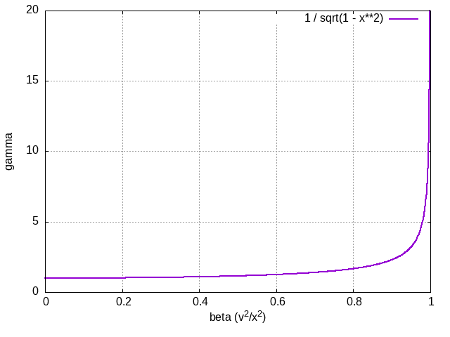
Figure 4.3.1 The lorenz factor as a function of \(\beta = v/c\). Note how it is close to 1 for most of the run, but grows out of control when \(v\) approaches the speed of light \(c\).

What insight does this give us on the energy of an object as it approaches the speed of light? Note that the formulae for length and time are:

\[\begin{split}L = \frac{1}{\gamma} L_0 \\ \Delta t' = \gamma \Delta t\end{split}\]

so the behavior of \(\gamma\) as a function of \(\beta\) (and thus \(v\)) also affects length and time.

Now let us look at the polynomial approximates in \(\beta\):

$ gnuplot
## then the following lines have the prompt gnuplot> and we type:
reset
set grid
set ylabel '\gamma'
set xlabel '\beta (v^2/c^2)'
set xrange [0:0.0001]
set terminal qt linewidth 3
plot 1 / (1 - x**2)
replot 1
replot 1 + (1.0/2) * x**2
replot 1 + (1.0/2) * x**2 + (3.0/8) * x**4
replot 1 + (1.0/2) * x**2 + (3.0/8) * x**4 + (5.0/16) * x**6